Academic Project in ARO3111 High Speed Aerodynamics
Contents
- Project Summary
- Tabulated Results
- Data Plots
- MATLAB Code Structure
- Hand Calculation Verification
- List of Symbols
- References
1.0 Project Summary
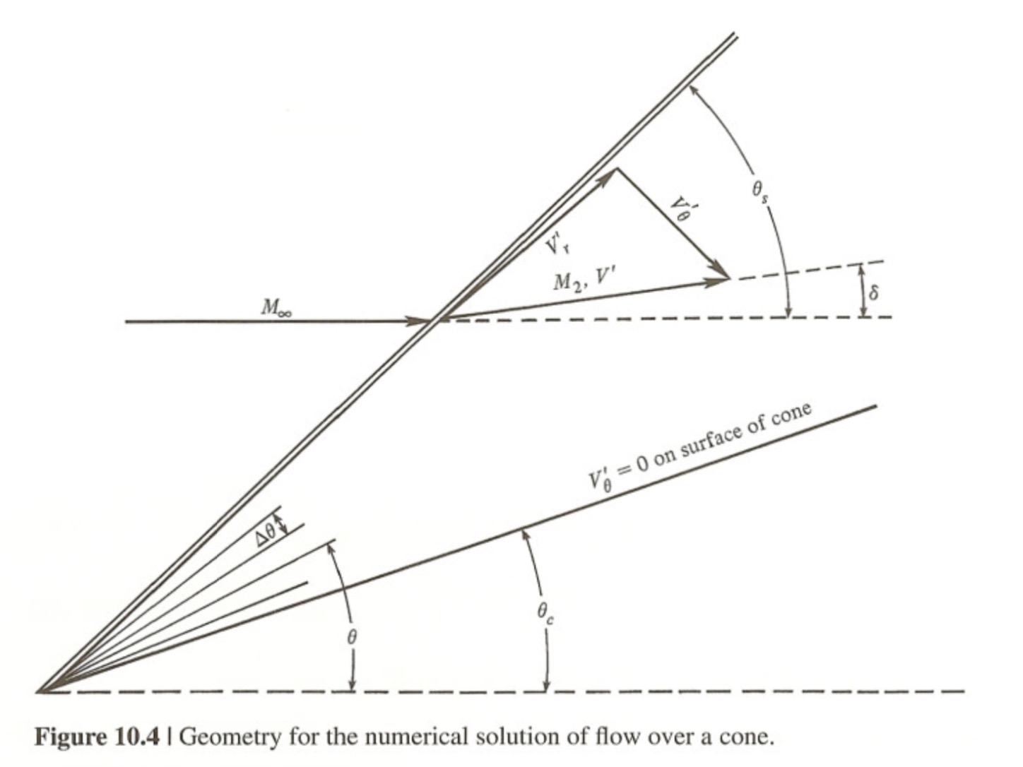
Conical flow is a vital concept that is analyzed because a majority of supersonic vehicles have some sort of sharp leading edge that can be approximated by a cone. The Taylor-Maccoll second order differential equation can be used to determine flow properties over a vertexed, right circular cone after an attached oblique shockwave, with the assumption of no yaw or pitch angle in an inviscid perfect gas. This equation was applied with a cylindrical coordinate system to determine the cone half-angle, static pressure, temperature, and density ratios across the shock, and the Mach number after the shock.
In order to model the Taylor-Maccoll equation and continue analysis by adding subsequent gas dynamics equations, MATLAB R2017A by Mathworks was utilized with a single script and multiple functions. Within the script file, the Runge-Kutta 4th Order differential equation solver was applied with a constant time step. This ensured solution accuracy, and the computation finished in a reasonable time. Further data analysis and manipulation was conducted in MATLAB and finally Microsoft Excel was used to compile the data. Below is the Taylor-Maccoll partial differential equation that is non-dimensionalized with respect to Vmax:
 (Modern Compressible Flow 3rd ed., Anderson Page 370)
The non-dimensionalized velocity equation is as follows:
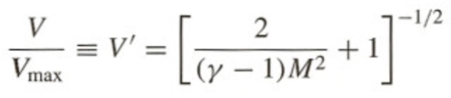 (Modern Compressible Flow 3rd ed., Anderson Page 371)
Taylor-Maccoll Test Case M = 2.0, Shock Angle = β=47°.
The computational process of the Taylor-Maccoll equation and flow past a cone begins by taking an input of the free stream Mach number (M1) and the shock angle (θs). Using oblique shock relations, the normal component of Mach before and after the shock and the Mach (M2) directly after the shock are calculated. Arrays of thetas were generated using the specified theta step (Δθ) (marching down from the shock angle to 0). Initial conditions to find the radial, angular, and total components of the velocity before and after the shock are then calculated. The initial Vr and Vθ at the shock is then passed to the 4th Order Runge-Kutta algorithm with specified functions of the derivative of the radial velocity and second derivative of the radial velocity to be solved.
A stopping condition of Vθ < 0 was incorporated to have the numerical differentiation stop when the theta reached the cone angle. The program generates two sets of arrays; one before the shock and one after the shock using the differential equation solver. In order to merge the two results together, a data processing section was added and this section also took the non-dimensional velocity (V’) and turned it into a Mach value (M). Gas dynamics was then applied to the Mach array to determine the ratio between the static pressure (P), temperature (T), and density (ρ) before and after the shock at varying theta angles (from the tip of the cone extending radially). This is done by dividing the static/total ratio over the static/total ratio from the local theta point over the Mach immediately behind the shock. This result is then multiplied to the ratio of static condition before and after the shock to get the final result – static condition locally over the static condition before the shock. Results generated for pressure, density, and temperature were included with Mach and theta angles and were both graphed and tabulated.
From the computed data, the change in static conditions are significant before and after the shock. These can be seen graphically as the shock is the vertical line jump in the plots. Also, in order to have greater solution accuracy, a small incremental theta step is required. The pressure ratio was the largest and then the density ratio and temperature ratio followed respectively. Overall, the results agree with the theory and hand calculations. The Taylor-Maccoll equation and 4th order Runge-Kutta algorithm allow for efficient and relatively accurate solutions to flow past an un-yawed cone.
2.0 Tabulated Results
Table 1.1 – Summary Theta, Velocity, Mach, Pressure, Temperature, and Density
| θ (deg.) | Vr/Vmax | Vθ/Vmax | Mach | Vmax | pc/p1 | Tc/T1 | ρc/ρ1 |
| 47 | 0.45466557 | -0.2711681 | 1.39530815 | 0.5293892 | 2.32943177 | 1.29554473 | 1.79803269 |
| 46.5 | 0.45699909 | -0.2636515 | 1.38876385 | 0.52759858 | 2.35094169 | 1.29895152 | 1.80987639 |
| 46 | 0.45926741 | -0.2562222 | 1.38259888 | 0.52590529 | 2.37134492 | 1.30216252 | 1.82108215 |
| 45.5 | 0.46147121 | -0.2488619 | 1.37676649 | 0.52429757 | 2.39077257 | 1.3052017 | 1.83172652 |
| 45 | 0.46361103 | -0.2415558 | 1.3712296 | 0.5227661 | 2.40932849 | 1.30808808 | 1.84187023 |
| 44.5 | 0.46568728 | -0.2342916 | 1.3659583 | 0.52130338 | 2.42709627 | 1.31083702 | 1.85156219 |
| 44 | 0.46770028 | -0.2270591 | 1.36092814 | 0.51990326 | 2.44414395 | 1.31346108 | 1.86084232 |
| 43.5 | 0.46965028 | -0.2198496 | 1.35611893 | 0.51856072 | 2.46052743 | 1.3159706 | 1.86974346 |
| 43 | 0.47153743 | -0.2126554 | 1.35151389 | 0.51727157 | 2.4762929 | 1.31837422 | 1.87829288 |
| 42.5 | 0.47336184 | -0.20547 | 1.34709897 | 0.51603233 | 2.4914787 | 1.32067915 | 1.88651324 |
| 42 | 0.47512356 | -0.1982874 | 1.34286237 | 0.51484009 | 2.50611661 | 1.32289144 | 1.89442349 |
| 41.5 | 0.4768226 | -0.1911024 | 1.3387942 | 0.51369242 | 2.52023295 | 1.32501617 | 1.90203939 |
| 41 | 0.47845891 | -0.1839099 | 1.33488615 | 0.51258732 | 2.53384936 | 1.32705762 | 1.90937403 |
| 40.5 | 0.4800324 | -0.1767055 | 1.33113128 | 0.51152314 | 2.54698338 | 1.32901934 | 1.91643816 |
| 40 | 0.48154295 | -0.1694849 | 1.32752386 | 0.51049852 | 2.559649 | 1.33090427 | 1.92324051 |
| 39.5 | 0.48299041 | -0.1622441 | 1.32405924 | 0.50951241 | 2.57185696 | 1.33271478 | 1.92978797 |
| 39 | 0.48437458 | -0.1549794 | 1.3207337 | 0.508564 | 2.58361506 | 1.33445279 | 1.93608577 |
| 38.5 | 0.48569523 | -0.1476868 | 1.31754441 | 0.5076527 | 2.59492841 | 1.33611973 | 1.94213763 |
| 38 | 0.48695211 | -0.1403629 | 1.31448935 | 0.50677815 | 2.60579954 | 1.33771664 | 1.94794583 |
| 37.5 | 0.48814492 | -0.1330038 | 1.31156727 | 0.5059402 | 2.61622854 | 1.33924412 | 1.95351131 |
| 37 | 0.48927335 | -0.1256061 | 1.30877765 | 0.5051389 | 2.62621309 | 1.34070244 | 1.95883367 |
| 36.5 | 0.49033704 | -0.118166 | 1.30612068 | 0.50437449 | 2.63574854 | 1.34209148 | 1.96391124 |
| 36 | 0.4913356 | -0.1106798 | 1.30359726 | 0.5036474 | 2.64482787 | 1.34341074 | 1.96874105 |
| 35.5 | 0.49226862 | -0.1031437 | 1.30120902 | 0.50295827 | 2.65344165 | 1.34465937 | 1.97331883 |
| 35 | 0.49313564 | -0.0955537 | 1.29895828 | 0.50230794 | 2.66157797 | 1.34583613 | 1.97763897 |
| 34.5 | 0.49393618 | -0.0879056 | 1.29684814 | 0.50169745 | 2.66922234 | 1.3469394 | 1.98169446 |
| 34 | 0.4946697 | -0.0801951 | 1.29488246 | 0.50112809 | 2.67635755 | 1.34796715 | 1.98547684 |
| 33.5 | 0.49533565 | -0.0724176 | 1.29306595 | 0.50060135 | 2.68296345 | 1.34891691 | 1.98897606 |
| 33 | 0.49593342 | -0.0645683 | 1.29140419 | 0.500119 | 2.68901678 | 1.34978577 | 1.99218042 |
| 32.5 | 0.49646236 | -0.0566419 | 1.28990374 | 0.49968308 | 2.69449089 | 1.35057028 | 1.9950764 |
| 32 | 0.49692177 | -0.0486329 | 1.2885722 | 0.49929591 | 2.69935538 | 1.35126648 | 1.99764845 |
| 31.5 | 0.4973109 | -0.0405353 | 1.28741836 | 0.49896016 | 2.70357578 | 1.35186976 | 1.99987887 |
| 31 | 0.49762896 | -0.0323425 | 1.28645228 | 0.49867888 | 2.70711304 | 1.35237488 | 2.0017475 |
| 30.5 | 0.49787509 | -0.0240474 | 1.28568545 | 0.4984555 | 2.70992305 | 1.35277581 | 2.00323145 |
| 30 | 0.49804835 | -0.0156424 | 1.28513104 | 0.49829393 | 2.71195596 | 1.35306568 | 2.00430474 |
| 29.5 | 0.49814775 | -0.0071188 | 1.28480405 | 0.49819862 | 2.7131555 | 1.35323665 | 2.00493794 |
| 29 | 0.49817222 | 0.00153281 | 1.28472161 | 0.49817458 | 2.71345799 | 1.35327975 | 2.0050976 |
3.0 Data Plots
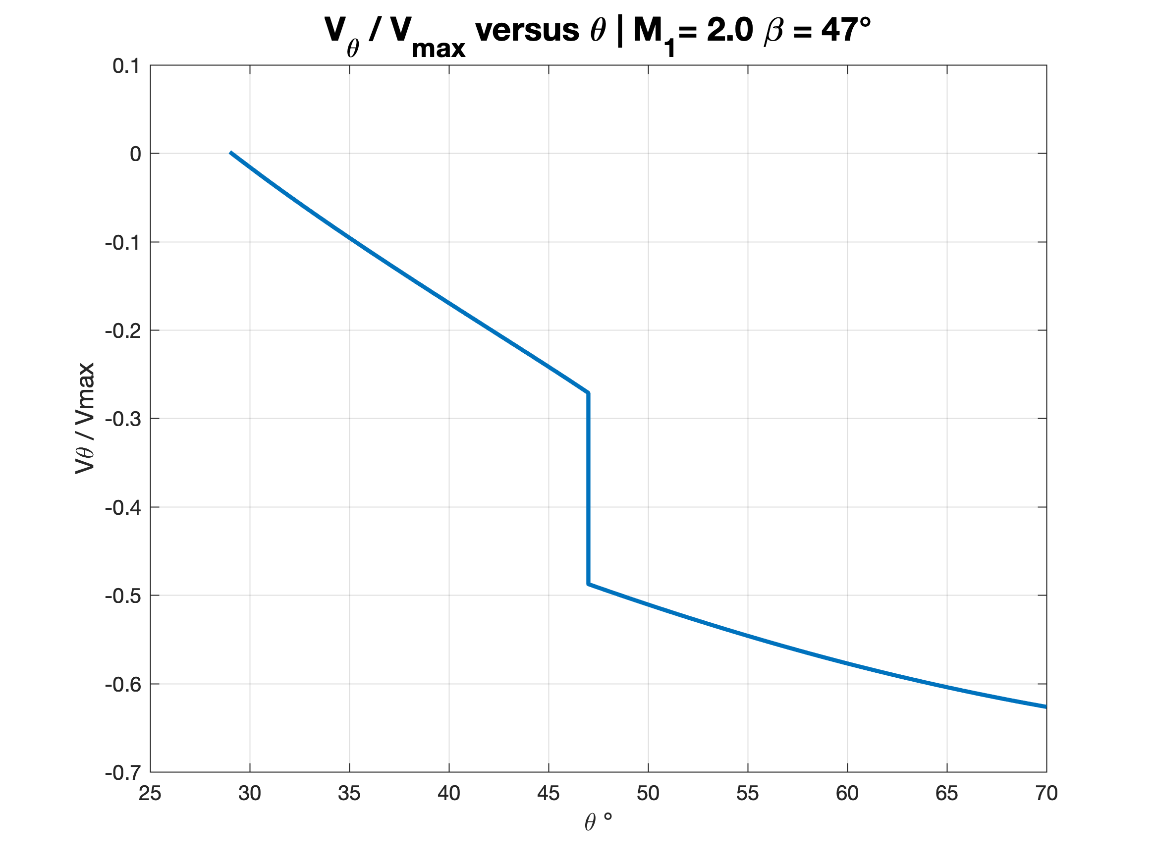
Figure 3.1 – Vθ/Vmax versus Theta | M1 = 2.0 β=47°
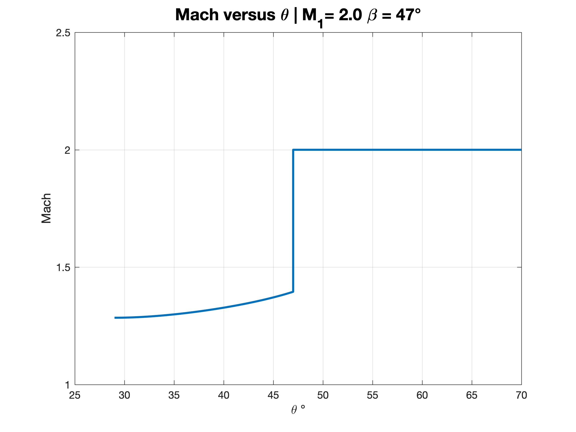
Figure 3.2 – Mach versus Theta | M1 = 2.0 β=47°

Figure 3.3 – Pressure, Density, and Temperature Ratios versus Theta | M1 = 2.0 β=47°
4.0 MATLAB Code Structure
| File Name | Contribution |
| flowpastcone_tm_rk4thode.m | (SCRIPT) User input goes here. Solves initial conditions, runs built in Runge-Kutta 4th Order ODE Solver, combines data from before and after shock and to cone angle, converts velocities into Mach, finds static pressure temperature and density ratios from before and after the shock, tabulates and stores final data into an array, plots and saves (.png) 3 figures seen above in the report. |
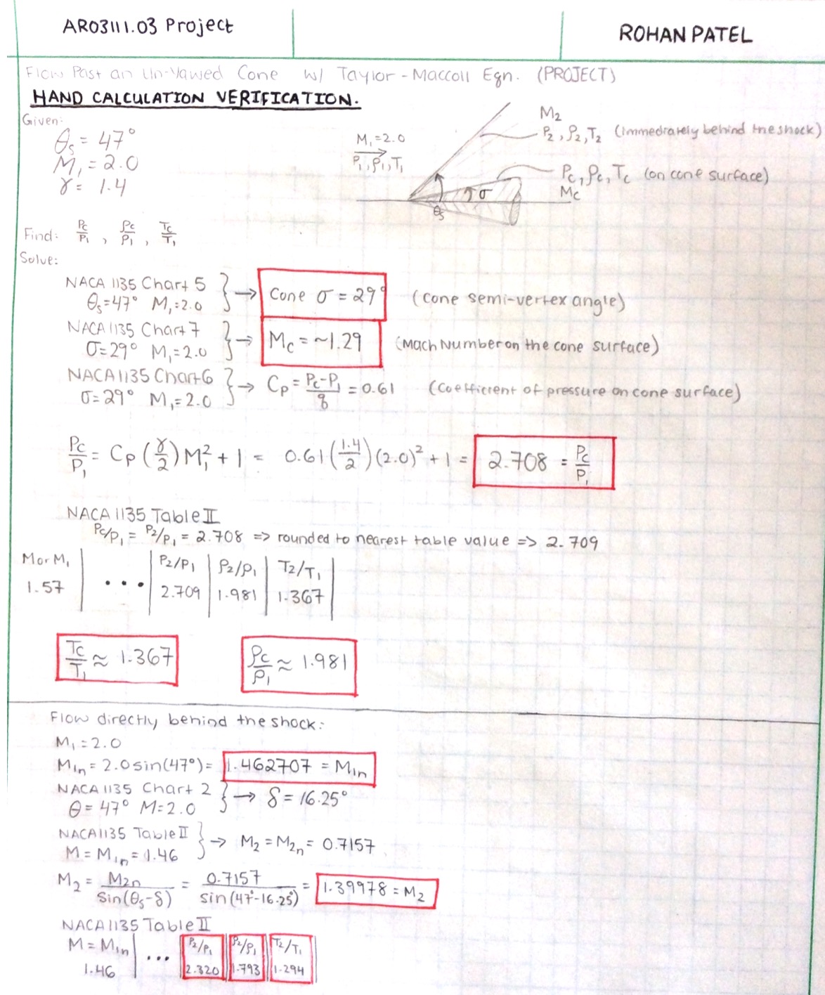
5.0 Hand Calculation Verification
6.0 List of Symbols
| θ – Angle measured from the horizontal (parallel to flow) |
| Δθ – Angle step size |
| θs – Shock Angle |
| θc – Cone Angle |
| M1 – Free Stream Mach |
| M2 – Mach Immediately After the Shock |
| V’ – Non-Dimensional Velocity |
| Vθ – Angular Velocity |
| Vr – Radial Velocity |
| ρ – Density |
| P– Pressure |
| T – Temperature |
| t subscript = total
1 subscript = free stream condition c subscript = cone surface condition |
7.0 References
- Aerodynamics Aeronautics and Flight Mechanics Barnes W. McCormick (2nd ed.)
- Modern Compressible Flow John D. Anderson (3th ed.)
- Dr. Tony Lin’s PowerPoint presentation on TM-Eqn and supersonic flow (in-Class)
- Dr. Ali Ahmadi’s handwritten notes on TM-Eqn (in-Class)